train_condition.py

import torch
import torch.nn as nn

from torchvision.utils import make_grid
from networks import make_grid as mkgrid

import argparse
import os
import time
from cp_dataset import CPDataset, CPDatasetTest, CPDataLoader
from networks import ConditionGenerator, VGGLoss, GANLoss, load_checkpoint, save_checkpoint, define_D
from tqdm import tqdm
from tensorboardX import SummaryWriter
from utils import *
from torch.utils.data import Subset

引入了很多库。

def iou_metric(y_pred_batch, y_true_batch):
    B = y_pred_batch.shape[0]
    iou = 0
    for i in range(B):
        y_pred = y_pred_batch[i]
        y_true = y_true_batch[i]
        # y_pred is not one-hot, so need to threshold it
        y_pred = y_pred > 0.5
        
        y_pred = y_pred.flatten()
        y_true = y_true.flatten()

    
        intersection = torch.sum(y_pred[y_true == 1])
        union = torch.sum(y_pred) + torch.sum(y_true)

    
        iou += (intersection + 1e-7) / (union - intersection + 1e-7) / B
    return iou

这个函数是用来计算IoU的，即Intersection Over Union，计算公式为 $$IoU = \frac{\text{Area of Intersection}}{\text{Area of Union}}$$

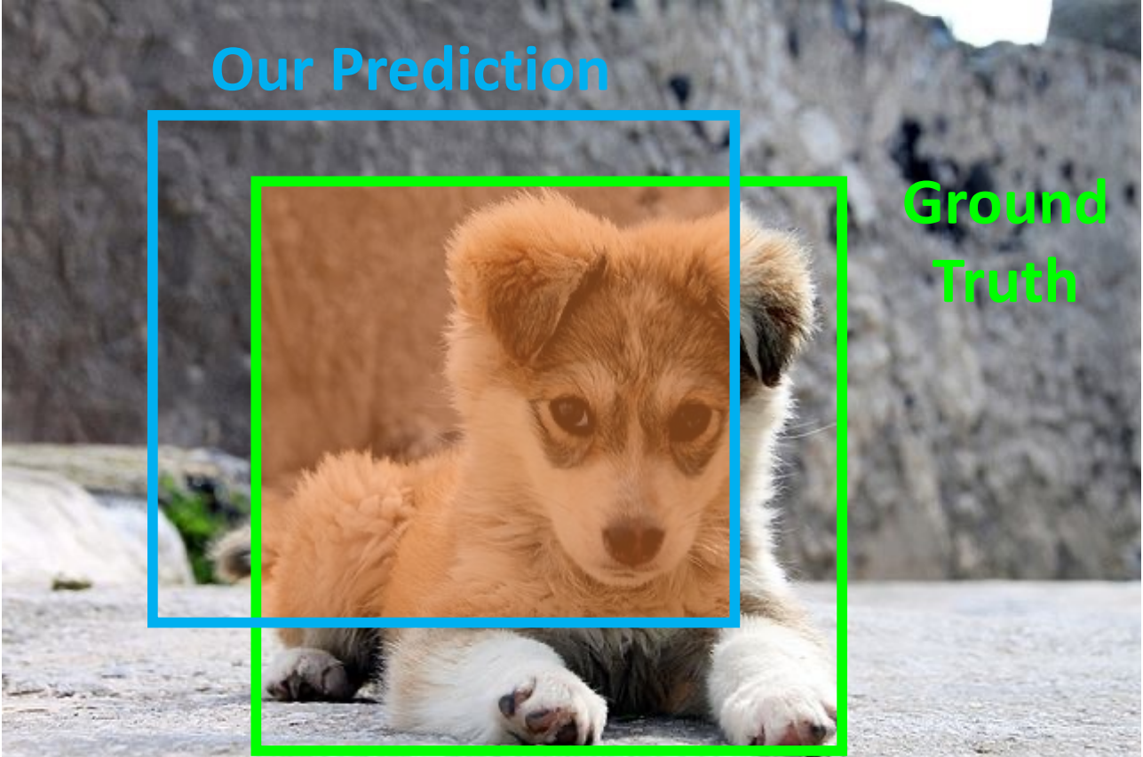
这里代码中分母用的是union - intersection的原因是，代码中的"union"不是真正的并集，而是把他们两个的区域面积直接加起来，多算了一次交集的面积，所以要减掉。

def remove_overlap(seg_out, warped_cm):
    
    assert len(warped_cm.shape) == 4
    
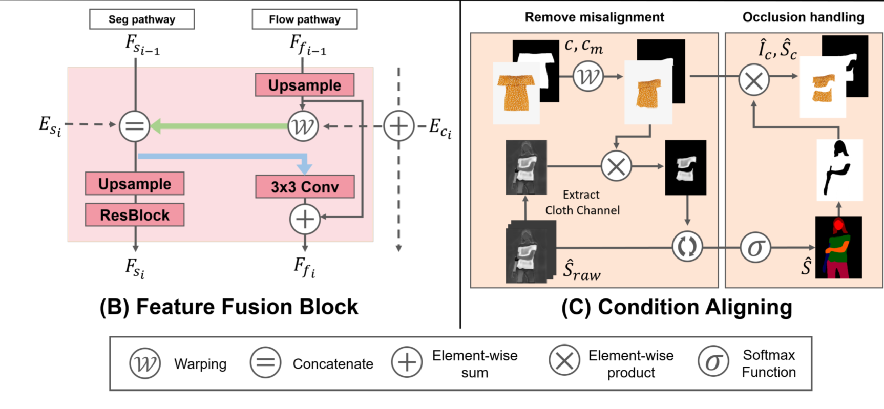
    warped_cm = warped_cm - (torch.cat([seg_out[:, 1:3, :, :], seg_out[:, 5:, :, :]], dim=1)).sum(dim=1, keepdim=True) * warped_cm
    return warped_cm

其中torch.cat([seg_out[:, 1:3, :, :], seg_out[:, 5:, :, :]], dim=1)表示segmentation中可能和clothes mask重叠的人体部位。

这里就是把warped clothes mask中和segmentation map中没对齐的部分消掉。看下面这张图就很清晰了。

def get_opt():
    parser = argparse.ArgumentParser()

    parser.add_argument("--name", default="test")
    parser.add_argument("--gpu_ids", default="")

	# omitted
	
    opt = parser.parse_args()
    return opt

然后是get_opt函数，从命令行中获取参数。

train

然后是训练的主体函数。HR-VITON在开源代码里提供了训练的细节，而VITON-HD根本没有关于训练的部分，可以作为一个很好的补充。

def train(opt, train_loader, test_loader, val_loader, board, tocg, D):
    # Model
    tocg.cuda() 
    tocg.train()
    D.cuda()
    D.train()

这里tocg指的是Try-On Condition Generator, D是Try-On Image Generator.

    # criterion
    criterionL1 = nn.L1Loss()
    criterionVGG = VGGLoss(opt)
    if opt.fp16:
        criterionGAN = GANLoss(use_lsgan=True, tensor=torch.cuda.HalfTensor)
    else :
        criterionGAN = GANLoss(use_lsgan=True, tensor=torch.cuda.FloatTensor if opt.gpu_ids else torch.Tensor)

    # optimizer
    optimizer_G = torch.optim.Adam(tocg.parameters(), lr=opt.G_lr, betas=(0.5, 0.999))
    optimizer_D = torch.optim.Adam(D.parameters(), lr=opt.D_lr, betas=(0.5, 0.999))

VGG Loss:

criterionVGG = VGGLoss(opt)：VGG损失是一种基于预训练的VGG网络的特征表示来计算的感知损失。它不仅比较像素值的差异，而且比较高级特征的差异，有助于生成视觉上更令人满意的结果。opt可能包含了配置VGG损失所需的特定选项或参数。

根据opt.fp16的设置，GAN损失可能使用半精度浮点数（torch.cuda.HalfTensor）以提高计算效率和降低内存使用，或者使用全精度浮点数（torch.cuda.FloatTensor）。opt.gpu_ids可能用来检查是否有GPU可用，如果没有，则使用默认的CPU tensor（torch.Tensor）。

optimizer_G = torch.optim.Adam(tocg.parameters(), lr=opt.G_lr, betas=(0.5, 0.999))：为生成器tocg设置Adam优化器。这里，lr=opt.G_lr是学习率，betas是Adam优化器的动量项，用于调节梯度下降过程中的移动平均。

for step in tqdm(range(opt.load_step, opt.keep_step)):
        iter_start_time = time.time()
        inputs = train_loader.next_batch()

这里tqdm是一个可以在控制台显示进度条的库。效果如下：

opt.load_step：可能表示模型加载时的起始步骤或迭代次数。在某些情况下，模型可能需要从先前训练的检查点继续训练，而 opt.load_step 就是指定了从哪一步开始加载模型的参数。
opt.keep_step：可能表示模型训练的结束步骤或迭代次数。当模型训练达到这个步骤时，循环就会结束。

然后就是用DataLoader加载数据集：

        # input1
        c_paired = inputs['cloth']['paired'].cuda()
        cm_paired = inputs['cloth_mask']['paired'].cuda()
        cm_paired = torch.FloatTensor((cm_paired.detach().cpu().numpy() > 0.5).astype(np.float)).cuda()
        # input2
        parse_agnostic = inputs['parse_agnostic'].cuda()
        densepose = inputs['densepose'].cuda()
        openpose = inputs['pose'].cuda()
        # GT
        label_onehot = inputs['parse_onehot'].cuda()  # CE
        label = inputs['parse'].cuda()  # GAN loss
        parse_cloth_mask = inputs['pcm'].cuda()  # L1
        im_c = inputs['parse_cloth'].cuda()  # VGG
        # visualization
        im = inputs['image']

        # inputs
        input1 = torch.cat([c_paired, cm_paired], 1)
        input2 = torch.cat([parse_agnostic, densepose], 1)

        # forward
        flow_list, fake_segmap, warped_cloth_paired, warped_clothmask_paired = tocg(input1, input2)
        
        # warped cloth mask one hot 
        
        warped_cm_onehot = torch.FloatTensor((warped_clothmask_paired.detach().cpu().numpy() > 0.5).astype(np.float)).cuda()

加载之后经过Try-On Condition Generator产生相应的结果。并把产生的warped_cm进行二值化处理。

这里的fake_segmap应该并不是说产生的segmentation map是有问题的，而是说这个segmentation map并不是来自于真实的图像，而是计算机合成的。

# fake segmap cloth channel * warped clothmask
   if opt.clothmask_composition != 'no_composition':
        if opt.clothmask_composition == 'detach':
            cloth_mask = torch.ones_like(fake_segmap.detach())
            cloth_mask[:, 3:4, :, :] = warped_cm_onehot
            fake_segmap = fake_segmap * cloth_mask

检查是否需要合成衣物掩码。如果 opt.clothmask_composition 不等于 'no_composition'，则表示需要进行衣物掩码的合成

opt.clothmask_composition == 'detach'：如果选择了使用 detach 方式合成衣物掩码，则将生成的虚假分割图 fake_segmap 与变形后的衣物掩码 warped_cm_onehot 相乘。这里使用 detach 可能是为了避免反向传播对 warped_cm_onehot 的影响。
opt.clothmask_composition == 'warp_grad'：如果选择了使用 warp_grad 方式合成衣物掩码，则将生成的虚假分割图 fake_segmap 与变形后的衣物掩码 warped_clothmask_paired 相乘。

if opt.occlusion:
    warped_clothmask_paired = remove_overlap(
        F.softmax(fake_segmap, dim=1), warped_clothmask_paired)
    warped_cloth_paired = warped_cloth_paired * warped_clothmask_paired + \
        torch.ones_like(warped_cloth_paired) * (1-warped_clothmask_paired)

这里是做occlusion handling。

调用remove_overlap把warped clothes mask与segmentation map中不重叠的部分消除掉，然后对warped_cloth也根据warped clothes mask把不重叠的地方消除掉。

warped_cloth_paired * warped_clothmask_paired让warped_clothmask_paired让未被遮挡的衣服保留下来，torch.ones_like(warped_cloth_paired) * (1-warped_clothmask_paired)为被遮挡的地方填充一个默认值（白色）。

fake_clothmask = (torch.argmax(fake_segmap.detach(), dim=1, keepdim=True) == 3).long()
misalign = fake_clothmask - warped_cm_onehot
misalign[misalign < 0.0] = 0.0

fake_clothmask = (torch.argmax(fake_segmap.detach(), dim=1, keepdim=True) == 3).long()这句话找出了在fake_segmap上最有可能是衣服的像素点，当做fake_clothmask。然后与ground truth相比，计算损失。

loss_l1_cloth = criterionL1(warped_clothmask_paired, parse_cloth_mask) 
loss_vgg = criterionVGG(warped_cloth_paired, im_c) 
loss_tv = 0

这里计算相应的损失。

首先计算了生成的clothmask和ground truth之间的 L1 Loss。

然后再计算了变形后的衣服与ground truth衣服之间的VGG Loss。

loss_tv先设置为0，下面再进行实际的运算。

        if opt.edgeawaretv == 'no_edge':
            if not opt.lasttvonly:
                for flow in flow_list:
                    y_tv = torch.abs(flow[:, 1:, :, :] - flow[:, :-1, :, :]).mean()
                    x_tv = torch.abs(flow[:, :, 1:, :] - flow[:, :, :-1, :]).mean()
                    loss_tv = loss_tv + y_tv + x_tv
            else:
                for flow in flow_list[-1:]:
                    y_tv = torch.abs(flow[:, 1:, :, :] - flow[:, :-1, :, :]).mean()
                    x_tv = torch.abs(flow[:, :, 1:, :] - flow[:, :, :-1, :]).mean()
                    loss_tv = loss_tv + y_tv + x_tv

这里是Total Variation Loss的计算。

这里flow的四个维度分别为$(N, H, W, C)$。

我们这里回忆一下图像梯度的计算公式： $$\frac{ \partial I(x,y) }{ \partial x } = \frac{I(x + 1, y) - I(x - 1,y)}{2}$$ $$\frac{ \partial I(x,y) }{ \partial y } = \frac{I(x, y + 1) - I(x,y-1)}{2}$$ 也可以写成： $$\frac{ \partial I(x,y) }{ \partial x } = \frac{I(x + 1, y) - I(x,y)}{1}$$ $$\frac{ \partial I(x,y) }{ \partial y } = \frac{I(x, y + 1) - I(x,y)}{1}$$

如果 opt.edgeawaretv 为 'no_edge' 且未指定 'lasttvonly':

对于每个流（flow）：
- 分别计算垂直方向（y_tv）和水平方向（x_tv）的像素变化的绝对值的平均值。
- 将这两个方向的总变差加到总的变差损失中。

flow[:, 1:, :, :]意思是取出2到n行，flow[:, :-1, :, :]意思是取出1到n-1行，两者作差即得到我们需要的n-1个对应上下两行的差，即第二行减第一行，第三行减第二行，……，第n行减第n-1行。

如果指定了'lasttvonly':

仅对最后一个流进行处理。
与上述类似，计算垂直和水平方向的像素变化绝对值的平均值。

这里的opt.edgeawaretv表示在计算total variation的时候是否考虑边缘的信息。如果只有最后一个光流考虑边缘的信息。

else:
			    if opt.edgeawaretv == 'last_only':
                flow = flow_list[-1]
                warped_clothmask_paired_down = F.interpolate(warped_clothmask_paired, flow.shape[1:3], mode='bilinear')
                y_tv = torch.abs(flow[:, 1:, :, :] - flow[:, :-1, :, :])
                x_tv = torch.abs(flow[:, :, 1:, :] - flow[:, :, :-1, :])
                mask_y = torch.exp(-15*torch.abs(0warped_clothmask_paired_down.permute(0, 2, 3, 1)[:, 1:, :, :] - warped_clothmask_paired_down.permute(0, 2, 3, 1)[:, :-1, :, :]))
                mask_x = torch.exp(-150*torch.abs(warped_clothmask_paired_down.permute(0, 2, 3, 1)[:, :, 1:, :] - warped_clothmask_paired_down.permute(0, 2, 3, 1)[:, :, :-1, :]))
                y_tv = y_tv * mask_y
                x_tv = x_tv * mask_x
                y_tv = y_tv.mean()
                x_tv = x_tv.mean()
                loss_tv = loss_tv + y_tv + x_tv

这里首先是跟上一步一样，计算了垂直方向（y_tv）和水平方向（x_tv）的像素变化的绝对值的平均值。

mask_y = torch.exp(-150*torch.abs(warped_clothmask_paired_down.permute(0, 2, 3, 1)[:, 1:, :, :] - warped_clothmask_paired_down.permute(0, 2, 3, 1)[:, :-1, :, :]))这个表达式，根据warped_clothmask_paired_down计算在垂直和水平方向上的像素变化幅度来计算mask_y。在变化幅度越大的地方权值越小。

因为在边缘区域，我们期望有更大的像素变化以保留边缘信息。通过这样的处理，梯度损失能更好地适应图像内容的具体情况，减少对边缘细节的平滑，这对于维持图像质量和视觉效果是非常重要的。

我们之后将这些计算出的边缘权重与原始的梯度值（y_tv 和 x_tv）相乘，并取平均值，得到最终的tv值。

elif opt.edgeawaretv == 'weighted':
                for i in range(5):
                    flow = flow_list[i]
                    warped_clothmask_paired_down = F.interpolate(warped_clothmask_paired, flow.shape[1:3], mode='bilinear')
                    y_tv = torch.abs(flow[:, 1:, :, :] - flow[:, :-1, :, :])
                    x_tv = torch.abs(flow[:, :, 1:, :] - flow[:, :, :-1, :])
                    mask_y = torch.exp(-150*torch.abs(warped_clothmask_paired_down.permute(0, 2, 3, 1)[:, 1:, :, :] - warped_clothmask_paired_down.permute(0, 2, 3, 1)[:, :-1, :, :]))
                    mask_x = torch.exp(-150*torch.abs(warped_clothmask_paired_down.permute(0, 2, 3, 1)[:, :, 1:, :] - warped_clothmask_paired_down.permute(0, 2, 3, 1)[:, :, :-1, :]))
                    y_tv = y_tv * mask_y
                    x_tv = x_tv * mask_x
                    y_tv = y_tv.mean() / (2 ** (4-i))
                    x_tv = x_tv.mean() / (2 ** (4-i))
                    loss_tv = loss_tv + y_tv + x_tv

如果opt.edgeawaretv == 'weighted'，这里的处理大体上和上面相似，只是上面只计算最后一个flow的TV值，而这里计算所有flow的TV值，并对他们进行加权。

使用 2 ** (4-i) 对不同阶段的损失进行动态加权，越晚的光流被赋予更大的权重，可能因为后期的图像变换更能代表整个图像序列的重要特征。

            if opt.add_lasttv:
                for flow in flow_list[-1:]:
                    y_tv = torch.abs(flow[:, 1:, :, :] - flow[:, :-1, :, :]).mean()
                    x_tv = torch.abs(flow[:, :, 1:, :] - flow[:, :, :-1, :]).mean()
                    loss_tv = loss_tv + y_tv + x_tv

最后如果add_lasttv为true，那么就加上最后一个flow的TV值。

if opt.interflowloss:
    for i in range(len(flow_list)-1):
        flow = flow_list[i]
        N, fH, fW, _ = flow.size()
        grid = mkgrid(N, iH, iW)
        flow = F.interpolate(flow.permute(0, 3, 1, 2), size=c_paired.shape[2:], mode=opt.upsample).permute(0, 2, 3, 1)
        flow_norm = torch.cat([flow[:, :, :, 0:1] / ((fW - 1.0) / 2.0), flow[:, :, :, 1:2] / ((fH - 1.0) / 2.0)], 3)
        warped_c = F.grid_sample(c_paired, flow_norm + grid, padding_mode='border')
        warped_cm = F.grid_sample(cm_paired, flow_norm + grid, padding_mode='border')
        warped_cm = remove_overlap(F.softmax(fake_segmap, dim=1), warped_cm)
        loss_l1_cloth += criterionL1(warped_cm, parse_cloth_mask) / (2 ** (4-i))
        loss_vgg += criterionVGG(warped_c, im_c) / (2 ** (4-i))

这里计算中间过程中的损失。同样是越后面的权重越大。

        # loss segmentation
        # generator
        CE_loss = cross_entropy2d(fake_segmap, label_onehot.transpose(0, 1)[0].long())

这里首先计算生成的segmentation map和实际的segmentation map之间的cross entropy loss。

在深度学习中，交叉熵损失函数常用于分类任务中。而在像素级的分类任务，比如图像语义分割，每个像素都需要分到一个类别中。使用独热编码的标签形式有几个好处：

方便计算： 独热编码的标签形式将标签表示为一个向量，其中只有一个元素是1，其余元素都是0。这样在计算损失时，只需要比较模型的输出与独热编码的标签，计算对应位置的交叉熵损失即可，计算起来相对简单高效。
适用性广泛： 独热编码的标签形式适用于多类别分类问题，可以处理类别不平衡的情况，每个类别的权重都可以独立地被考虑。
数学上的连续性： 交叉熵损失函数可以直接衡量两个概率分布之间的差异，而独热编码的标签形式与概率分布形式相对应，这使得交叉熵损失函数的数学解释更加直观。

这里的cross_entropy2d是在utils.py中定义的，并不是一个内置的函数。

def cross_entropy2d(input, target, weight=None, size_average=True):
    n, c, h, w = input.size()
    nt, ht, wt = target.size()

    # Handle inconsistent size between input and target
    if h != ht or w != wt:
        input = F.interpolate(input, size=(ht, wt), mode="bilinear", align_corners=True)

    input = input.transpose(1, 2).transpose(2, 3).contiguous().view(-1, c)
    target = target.view(-1)
    loss = F.cross_entropy(
        input, target, weight=weight, size_average=size_average, ignore_index=250
    )
    return loss

首先取出了input和target的形状。如果input和target的形状不同，就进行缩放处理。

input.transpose(1, 2).transpose(2, 3).contiguous() 将输入张量从 (N, C, H, W) 转换为 (N, H, W, C)。便于之后的展平。

这里我们回忆一下view的用法： view 方法用于改变张量的形状而不改变其数据。你可以将其视为重新排列或解释张量中数据的一种方式，但实际的数据内容和顺序不变。这通常用于调整数据的维度以匹配特定操作或模型的输入需求。

使用场景：例如，如果你有一个形状为 [10, 256] 的张量，你可以使用 .view(10, 16, 16) 将其重新形状为 [10, 16, 16]，这样做是为了将它用作图像批次，其中每张图像是 16x16 像素。
限制：使用 view 需要张量在内存中是连续的（即无跨步问题）。如果不是，可能需要先调用 .contiguous()。
自动推断维度：用 -1 作为 view 方法中的一个参数，PyTorch 将自动计算这一维的大小，以使得总元素数量保持不变。

F.cross_entropy(input, target, weight=weight, size_average=size_average, ignore_index=250) 使用 PyTorch 提供的交叉熵函数计算损失。ignore_index=250 参数指示函数忽略值为 250 的目标标签，这通常用于表示某些像素不应该被计算损失（例如，标注不清的区域）。

现在我们再回过头来看刚才的CE Loss计算。

CE_loss = cross_entropy2d(fake_segmap, label_onehot.transpose(0, 1)[0].long())

label_onehot的维度为(N, 1, H, W)，这样然后调用transpose转化为(1, N, H, W)，最后把第一维去掉，得到(N, H, W)，符合cross_entropy2d函数的要求。

        if opt.no_GAN_loss:
            loss_G = (10 * loss_l1_cloth + loss_vgg + opt.tvlambda * loss_tv) + (CE_loss * opt.CElamda)
            # step
            optimizer_G.zero_grad()
            loss_G.backward()
            optimizer_G.step()

optimizer_G.zero_grad(): 这一步是将生成器的梯度缓存清零。在PyTorch中，梯度是累积的，因此在每次反向传播之前需要将梯度清零，以避免梯度的累积影响下一次的计算。
loss_G.backward(): 这一步是执行反向传播，计算生成器损失 loss_G 对生成器参数的梯度。反向传播会沿着计算图反向传播误差，并计算每个参数对总体损失的贡献度。
optimizer_G.step(): 这一步是利用优化器 optimizer_G 根据生成器参数的梯度更新参数值。优化器根据梯度和设定的优化算法（如随机梯度下降）更新参数，以减小损失函数的值，从而使生成器更好地生成符合期望的输出。

else:
            fake_segmap_softmax = torch.softmax(fake_segmap, 1)

            pred_segmap = D(torch.cat((input1.detach(), input2.detach(), fake_segmap_softmax), dim=1))
            
            loss_G_GAN = criterionGAN(pred_segmap, True)

这里是如果要加入GANLoss的操作。

pred_segmap = D(torch.cat((input1.detach(), input2.detach(), fake_segmap_softmax), dim=1))：这一步将经过softmax处理后的生成器输出与输入图像以及其他信息（如输入的衣服图像）进行拼接，然后输入到鉴别器 D 中进行预测。预测得到的 pred_segmap 是鉴别器对合成图像的预测结果。

loss_G_GAN = criterionGAN(pred_segmap, True)表示Generator希望它被判定为真实的。并计算相应的loss。

if not opt.G_D_seperate:
    # discriminator
    fake_segmap_pred = D(torch.cat((input1.detach(), input2.detach(), fake_segmap_softmax.detach()), dim=1))
    real_segmap_pred = D(torch.cat((input1.detach(), input2.detach(), label), dim=1))
    loss_D_fake = criterionGAN(fake_segmap_pred, False)
    loss_D_real = criterionGAN(real_segmap_pred, True)

    # loss sum
    loss_G = (10 * loss_l1_cloth + loss_vgg + opt.tvlambda * loss_tv) + (
                CE_loss * opt.CElamda + loss_G_GAN * opt.GANlambda)  # warping + seg_generation
    loss_D = loss_D_fake + loss_D_real

    # step
    optimizer_G.zero_grad()
    loss_G.backward()
    optimizer_G.step()

    optimizer_D.zero_grad()
    loss_D.backward()
    optimizer_D.step()

如果Generator和Discriminator不分开训练，那么就再计算Discriminator的Loss，然后计算Generator的总Loss。然后调用optimizer进行优化。

这里将真实的input和fake_segmap一起作为fake_segmap_pred可能是因为将真实数据与生成数据一起输入判别器可以帮助判别器更好地学习如何区分真实数据和生成数据。

fake_segmap_pred = D(torch.cat((input1.detach(), input2.detach(), fake_segmap_softmax.detach()), dim=1))这句使用 detach 函数将生成器输出的梯度信息从计算图中分离出来，以防止梯度更新传播到生成器，从而保持生成器参数不变。

else: # train G first after that train D
                # loss G sum
                loss_G = (10 * loss_l1_cloth + loss_vgg + opt.tvlambda * loss_tv) + (CE_loss * opt.CElamda + loss_G_GAN * opt.GANlambda)  # warping + seg_generation
                
                # step G
                optimizer_G.zero_grad()
                loss_G.backward()
                optimizer_G.step()
                
                # discriminator
                with torch.no_grad():
                    _, fake_segmap, _, _ = tocg(input1, input2)
                fake_segmap_softmax = torch.softmax(fake_segmap, 1)
                
                # loss discriminator
                fake_segmap_pred = D(torch.cat((input1.detach(), input2.detach(), fake_segmap_softmax.detach()),dim=1))
                real_segmap_pred = D(torch.cat((input1.detach(), input2.detach(), label),dim=1))
                loss_D_fake = criterionGAN(fake_segmap_pred, False)
                loss_D_real = criterionGAN(real_segmap_pred, True)
                
                loss_D = loss_D_fake + loss_D_real
                
                optimizer_D.zero_grad()
                loss_D.backward()
                optimizer_D.step()

如果opt.G_D_seperate == True，就先训练Generator，再训练Discriminator。

if (step + 1) % opt.val_count == 0:  
    tocg.eval()  
    iou_list = []  
    with torch.no_grad():  
        for cnt in range(2000 // opt.batch_size):  
  
            inputs = val_loader.next_batch()  
            # input1  
            c_paired = inputs['cloth']['paired'].cuda()  
            cm_paired = inputs['cloth_mask']['paired'].cuda()  
            cm_paired = torch.FloatTensor((cm_paired.detach().cpu().numpy() > 0.5).astype(np.float)).cuda()  
            # input2  
            parse_agnostic = inputs['parse_agnostic'].cuda()  
            densepose = inputs['densepose'].cuda()  
            openpose = inputs['pose'].cuda()  
            # GT  
            label_onehot = inputs['parse_onehot'].cuda()  # CE  
            label = inputs['parse'].cuda()  # GAN loss  
            parse_cloth_mask = inputs['pcm'].cuda()  # L1  
            im_c = inputs['parse_cloth'].cuda()  # VGG  
            # visualization            im = inputs['image']  
  
            input1 = torch.cat([c_paired, cm_paired], 1)  
            input2 = torch.cat([parse_agnostic, densepose], 1)

if (step + 1) % opt.val_count == 0:每隔一段时间对模型进行一次评估。

tocg.eval()将模型设置为评估模式，这会影响到某些层的行为，例如Dropout和Batch Normalization层，在评估模式下会采用不同的统计信息，以便更好地进行评估。

通过torch.no_grad()上下文管理器，禁用梯度计算，因为在验证过程中不需要计算梯度，这样可以减少内存的使用并提高计算速度。

接着循环遍历验证集，每次加载一个批次的数据，然后将数据传输到GPU上（如果可用）。

# forward
flow_list, fake_segmap, warped_cloth_paired, warped_clothmask_paired = tocg(input1, input2)  
  
# fake segmap cloth channel * warped clothmask  
if opt.clothmask_composition != 'no_composition':  
    if opt.clothmask_composition == 'detach':  
        cloth_mask = torch.ones_like(fake_segmap.detach())  
        cloth_mask[:, 3:4, :, :] = warped_cm_onehot  
        fake_segmap = fake_segmap * cloth_mask  
  
    if opt.clothmask_composition == 'warp_grad':  
        cloth_mask = torch.ones_like(fake_segmap.detach())  
        cloth_mask[:, 3:4, :, :] = warped_clothmask_paired  
        fake_segmap = fake_segmap * cloth_mask  
  
# calculate iou  
iou = iou_metric(F.softmax(fake_segmap, dim=1).detach(), label)  
iou_list.append(iou.item())  
  
tocg.train()  
board.add_scalar('val/iou', np.mean(iou_list), step + 1)

下面是board.add_scalar函数的各个参数的解释： 'val/iou'：标签，用于标识被记录的数据类型，以便在tensorboard中显示。 np.mean(iou_list)：要记录的数值，这里是平均的IoU值。 step + 1：当前的步数，用于在tensorboard中横轴显示，以便对应模型训练的进度。

这里+1是因为循环的step从0开始，但是对于我们人类来说step从1开始更直观，所以我们+1。

Tensorboard是一个由Google开发的用于可视化神经网络训练过程中的各种指标和结果的工具。它可以帮助用户更直观地理解模型的训练过程和性能表现。在Tensorboard中，用户可以查看训练过程中的损失函数曲线、准确率曲线、模型参数分布、模型结构等信息，以及进行多组数据的对比分析。通过可视化，用户可以更好地监控模型的训练过程，发现潜在问题，并优化模型的训练策略。

# tensorboard  
if (step + 1) % opt.tensorboard_count == 0:  
    # loss G  
    board.add_scalar('Loss/G', loss_G.item(), step + 1)  
    board.add_scalar('Loss/G/l1_cloth', loss_l1_cloth.item(), step + 1)  
    board.add_scalar('Loss/G/vgg', loss_vgg.item(), step + 1)  
    board.add_scalar('Loss/G/tv', loss_tv.item(), step + 1)  
    board.add_scalar('Loss/G/CE', CE_loss.item(), step + 1)  
    if not opt.no_GAN_loss:  
        board.add_scalar('Loss/G/GAN', loss_G_GAN.item(), step + 1)  
        # loss D  
        board.add_scalar('Loss/D', loss_D.item(), step + 1)  
        board.add_scalar('Loss/D/pred_real', loss_D_real.item(), step + 1)  
        board.add_scalar('Loss/D/pred_fake', loss_D_fake.item(), step + 1)  
  
    grid = make_grid(  
        [(c_paired[0].cpu() / 2 + 0.5), (cm_paired[0].cpu()).expand(3, -1, -1), visualize_segmap(parse_agnostic.cpu()),  
         ((densepose.cpu()[0] + 1) / 2),  
         (im_c[0].cpu() / 2 + 0.5), parse_cloth_mask[0].cpu().expand(3, -1, -1),  
         (warped_cloth_paired[0].cpu().detach() / 2 + 0.5), (warped_cm_onehot[0].cpu().detach()).expand(3, -1, -1),  
         visualize_segmap(label.cpu()), visualize_segmap(fake_segmap.cpu()), (im[0] / 2 + 0.5),  
         (misalign[0].cpu().detach()).expand(3, -1, -1)],  
        nrow=4)  
    board.add_images('train_images', grid.unsqueeze(0), step + 1)

然后这段代码是在tensorboard里面记录一些其他的数据。

这里用的是torchvision库中的make_grid函数，而不是用的先前自己定义的。

make_grid 函数是 PyTorch 中用于将一组图像排列成一个网格的工具函数。它接受一个张量列表作为输入，这些张量通常代表一组图像。下面是它的部分参数：

tensor (list of tensors): 这是包含图像的张量列表。每个张量都代表一张图像，通常是 (C, H, W) 形状的张量，其中 C 是通道数，H 是高度，W 是宽度。这些张量可以具有不同的形状，但是它们的通道数必须相同。如果输入的张量是 [N, C, H, W] 形状的，make_grid 函数会将它们合并成一个 (C, H, W * N) 的张量，其中 N 是输入张量的数量。
nrow (int, optional): 这是一个可选参数，用于指定生成的网格中每行包含的图像数量。默认值为 8。
padding (int, optional): 这也是一个可选参数，用于指定每个图像之间的填充像素数。默认值为 2。
normalize (bool, optional): 这是一个可选参数，用于指定是否对输入张量进行归一化。如果设置为 True，则会对输入张量进行归一化，使其像素值范围在 [0, 1] 内。默认值为 False。
value (float, optional): 这是一个可选参数，用于指定填充像素的值。默认值为 0。

    if not opt.no_test_visualize:  
        inputs = test_loader.next_batch()  
        # input1  
        c_paired = inputs['cloth'][opt.test_datasetting].cuda()  
        cm_paired = inputs['cloth_mask'][opt.test_datasetting].cuda()  
        cm_paired = torch.FloatTensor((cm_paired.detach().cpu().numpy() > 0.5).astype(np.float)).cuda()  
        # input2  
        parse_agnostic = inputs['parse_agnostic'].cuda()  
        densepose = inputs['densepose'].cuda()  
        openpose = inputs['pose'].cuda()  
        # GT  
        label_onehot = inputs['parse_onehot'].cuda()  # CE  
        label = inputs['parse'].cuda()  # GAN loss  
        parse_cloth_mask = inputs['pcm'].cuda()  # L1  
        im_c = inputs['parse_cloth'].cuda()  # VGG  
        # visualization        im = inputs['image']  
  
        tocg.eval()

如果不是no_test_visualize的话，

if not opt.no_test_visualize:  
    inputs = test_loader.next_batch()  
    # input1  
    c_paired = inputs['cloth'][opt.test_datasetting].cuda()  
    cm_paired = inputs['cloth_mask'][opt.test_datasetting].cuda()  
    cm_paired = torch.FloatTensor((cm_paired.detach().cpu().numpy() > 0.5).astype(np.float)).cuda()  
    # input2  
    parse_agnostic = inputs['parse_agnostic'].cuda()  
    densepose = inputs['densepose'].cuda()  
    openpose = inputs['pose'].cuda()  
    # GT  
    label_onehot = inputs['parse_onehot'].cuda()  # CE  
    label = inputs['parse'].cuda()  # GAN loss  
    parse_cloth_mask = inputs['pcm'].cuda()  # L1  
    im_c = inputs['parse_cloth'].cuda()  # VGG  
    # visualization    im = inputs['image']  
  
    tocg.eval()  
    with torch.no_grad():  
        # inputs  
        input1 = torch.cat([c_paired, cm_paired], 1)  
        input2 = torch.cat([parse_agnostic, densepose], 1)  
  
        # forward  
        flow_list, fake_segmap, warped_cloth_paired, warped_clothmask_paired = tocg(input1, input2)  
  
        warped_cm_onehot = torch.FloatTensor(  
            (warped_clothmask_paired.detach().cpu().numpy() > 0.5).astype(np.float)).cuda()  
        if opt.clothmask_composition != 'no_composition':  
            if opt.clothmask_composition == 'detach':  
                cloth_mask = torch.ones_like(fake_segmap)  
                cloth_mask[:, 3:4, :, :] = warped_cm_onehot  
                fake_segmap = fake_segmap * cloth_mask  
  
            if opt.clothmask_composition == 'warp_grad':  
                cloth_mask = torch.ones_like(fake_segmap)  
                cloth_mask[:, 3:4, :, :] = warped_clothmask_paired  
                fake_segmap = fake_segmap * cloth_mask  
        if opt.occlusion:  
            warped_clothmask_paired = remove_overlap(F.softmax(fake_segmap, dim=1), warped_clothmask_paired)  
            warped_cloth_paired = warped_cloth_paired * warped_clothmask_paired + torch.ones_like(  
                warped_cloth_paired) * (1 - warped_clothmask_paired)  
  
        # generated fake cloth mask & misalign mask  
        fake_clothmask = (torch.argmax(fake_segmap.detach(), dim=1, keepdim=True) == 3).long()  
        misalign = fake_clothmask - warped_cm_onehot  
        misalign[misalign < 0.0] = 0.0  
  
    for i in range(opt.num_test_visualize):  
        grid = make_grid([(c_paired[i].cpu() / 2 + 0.5), (cm_paired[i].cpu()).expand(3, -1, -1),  
                          visualize_segmap(parse_agnostic.cpu(), batch=i), ((densepose.cpu()[i] + 1) / 2),  
                          (im_c[i].cpu() / 2 + 0.5), parse_cloth_mask[i].cpu().expand(3, -1, -1),  
                          (warped_cloth_paired[i].cpu().detach() / 2 + 0.5),  
                          (warped_cm_onehot[i].cpu().detach()).expand(3, -1, -1),  
                          visualize_segmap(label.cpu(), batch=i), visualize_segmap(fake_segmap.cpu(), batch=i),  
                          (im[i] / 2 + 0.5), (misalign[i].cpu().detach()).expand(3, -1, -1)],  
                         nrow=4)  
        board.add_images(f'test_images/{i}', grid.unsqueeze(0), step + 1)  
    tocg.train()

这段代码和上面的差不多，只是做的是test时候的visualization。这个train函数训练到一定的时候，不仅会看看在训练集上的效果，还会加载一些测试集的数据来评估一下。

# display  
if (step + 1) % opt.display_count == 0:  
    t = time.time() - iter_start_time  
    if not opt.no_GAN_loss:  
        print(  
            "step: %8d, time: %.3f\nloss G: %.4f, L1_cloth loss: %.4f, VGG loss: %.4f, TV loss: %.4f CE: %.4f, G GAN: %.4f\nloss D: %.4f, D real: %.4f, D fake: %.4f"  
            % (step + 1, t, loss_G.item(), loss_l1_cloth.item(), loss_vgg.item(), loss_tv.item(), CE_loss.item(),  
               loss_G_GAN.item(), loss_D.item(), loss_D_real.item(), loss_D_fake.item()), flush=True)  
  
# save  
if (step + 1) % opt.save_count == 0:  
    save_checkpoint(tocg, os.path.join(opt.checkpoint_dir, opt.name, 'tocg_step_%06d.pth' % (step + 1)), opt)  
    save_checkpoint(D, os.path.join(opt.checkpoint_dir, opt.name, 'D_step_%06d.pth' % (step + 1)), opt)

这部分代码是用于在训练过程中进行显示和保存操作。

显示（Display）：当达到一定的步数间隔时，通过 opt.display_count 控制，会打印当前训练的一些信息，例如损失值、当前步数、训练时间等，以便实时监控训练过程中的情况。这可以帮助调试和监控模型的训练过程。
保存（Save）：当达到一定的步数间隔时，通过 opt.save_count 控制，会保存当前的模型参数到文件中。这样可以定期保存模型的状态，以便在需要时进行恢复或者继续训练。

然后就是调用train的main函数，就没什么特别的了：

def main():
    opt = get_opt()
    print(opt)
    print("Start to train %s!" % opt.name)
    os.environ["CUDA_VISIBLE_DEVICES"] = opt.gpu_ids
    
    # create train dataset & loader
    train_dataset = CPDataset(opt)
    train_loader = CPDataLoader(opt, train_dataset)
    
    # create test dataset & loader
    test_loader = None
    if not opt.no_test_visualize:
        train_bsize = opt.batch_size
        opt.batch_size = opt.num_test_visualize
        opt.dataroot = opt.test_dataroot
        opt.datamode = 'test'
        opt.data_list = opt.test_data_list
        test_dataset = CPDatasetTest(opt)
        opt.batch_size = train_bsize
        val_dataset = Subset(test_dataset, np.arange(2000))
        test_loader = CPDataLoader(opt, test_dataset)
        val_loader = CPDataLoader(opt, val_dataset)
    # visualization
    if not os.path.exists(opt.tensorboard_dir):
        os.makedirs(opt.tensorboard_dir)
    board = SummaryWriter(log_dir=os.path.join(opt.tensorboard_dir, opt.name))

    # Model
    input1_nc = 4  # cloth + cloth-mask
    input2_nc = opt.semantic_nc + 3  # parse_agnostic + densepose
    tocg = ConditionGenerator(opt, input1_nc=4, input2_nc=input2_nc, output_nc=opt.output_nc, ngf=96, norm_layer=nn.BatchNorm2d)
    D = define_D(input_nc=input1_nc + input2_nc + opt.output_nc, Ddownx2 = opt.Ddownx2, Ddropout = opt.Ddropout, n_layers_D=3, spectral = opt.spectral, num_D = opt.num_D)
    
    # Load Checkpoint
    if not opt.tocg_checkpoint == '' and os.path.exists(opt.tocg_checkpoint):
        load_checkpoint(tocg, opt.tocg_checkpoint)

    # Train
    train(opt, train_loader, val_loader, test_loader, board, tocg, D)

    # Save Checkpoint
    save_checkpoint(tocg, os.path.join(opt.checkpoint_dir, opt.name, 'tocg_final.pth'),opt)
    save_checkpoint(D, os.path.join(opt.checkpoint_dir, opt.name, 'D_final.pth'),opt)
    print("Finished training %s!" % opt.name)


if __name__ == "__main__":
    main()

train_generator.py

def get_opt():
    parser = argparse.ArgumentParser()

    parser.add_argument('--name', type=str, required=True)
    parser.add_argument('--gpu_ids', type=str, default='0')

	# detailes omitted

    opt = parser.parse_args()

    # set gpu ids
    str_ids = opt.gpu_ids.split(',')
    opt.gpu_ids = []
    for str_id in str_ids:
        id = int(str_id)
        if id >= 0:
            opt.gpu_ids.append(id)
    if len(opt.gpu_ids) > 0:
        torch.cuda.set_device(opt.gpu_ids[0])

    assert len(opt.gpu_ids) == 0 or opt.batch_size % len(opt.gpu_ids) == 0, \
        "Batch size %d is wrong. It must be a multiple of # GPUs %d." \
        % (opt.batch_size, len(opt.gpu_ids))

    return opt

这里还是调用parser来获取用户的参数。

def train(opt, train_loader, test_loader, test_vis_loader, board, tocg, generator, discriminator, model):  
    # Model  
    if not opt.GT:  
        tocg.cuda()  
        tocg.eval()  
    generator.train()  
    discriminator.train()  
    model.eval()

这里opt.GT控制是使用真实的数据（segmentation map）训练还是使用tocg生成的segmentation map进行训练。

# criterion  
if opt.fp16:  
    criterionGAN = GANLoss('hinge', tensor=torch.cuda.HalfTensor)  
else:  
    criterionGAN = GANLoss('hinge', tensor=torch.cuda.FloatTensor)  
# criterionL1 = nn.L1Loss()  
criterionFeat = nn.L1Loss()  
criterionVGG = VGGLoss(opt)  
  
# optimizer  
optimizer_gen = torch.optim.Adam(generator.parameters(), lr=opt.G_lr, betas=(0, 0.9))  
scheduler_gen = torch.optim.lr_scheduler.LambdaLR(optimizer_gen, lr_lambda=lambda step: 1.0 -  max(0,step * 1000 + opt.load_step - opt.keep_step) / float(opt.decay_step + 1))  

optimizer_dis = torch.optim.Adam(discriminator.parameters(), lr=opt.D_lr, betas=(0, 0.9))  
scheduler_dis = torch.optim.lr_scheduler.LambdaLR(optimizer_dis, lr_lambda=lambda step: 1.0 -  max(0, step * 1000 + opt.load_step - opt.keep_step) / float(opt.decay_step + 1))

这里使用hinge loss。

这里还使用了学习率调度器（scheduler）。在深度学习训练过程中，学习率调度器（scheduler）是用来调整优化器的学习率的工具，以便控制训练过程中的学习速度。在这段代码中，使用的是 torch.optim.lr_scheduler.LambdaLR 调度器。这个调度器通过一个 lambda 函数来自定义学习率的调整策略，这提供了很大的灵活性。

这里的学习率调整策略为 $$\lambda(\text{step}) = 1.0 - \frac{\max(0, \text{step} \times 1000 + \text{opt.load_step} - \text{opt.keep_step})}{\text{opt.decay_step} + 1}$$ 公式分析： 参数的含义：

opt.load_step

含义：opt.load_step 通常指的是从哪一个训练步骤开始加载模型继续训练。这个参数在恢复中断的训练或从预训练模型开始训练时特别有用。它表示已经执行的训练步骤数，用于确保学习率调度和其他训练逻辑可以从正确的时间点开始。

opt.keep_step

含义：opt.keep_step 是指在训练过程中保持初始学习率不变的步数。换句话说，这是一个阈值，直到该步数之前，学习率将保持为开始时设置的初始值。
作用：通过设定一个初始阶段在该步数内不改变学习率，可以让模型在训练初期快速下降到一个合理的损失水平。在很多优化任务中，初期使用较高的固定学习率可以帮助模型跳出不良的局部最小值，或更快地接近全局最小值。

opt.decay_step

含义：opt.decay_step 定义了从 opt.keep_step 计算起，学习率需要经过多少步骤减少到0或接近0的一个阈值。它是学习率开始衰减后，直到衰减结束的步数总和。
作用：这个参数控制了学习率衰减的速度和持续时间。较大的 decay_step 值意味着学习率将以较慢的速度减少，这可能有助于模型在接近优化问题的解时进行更细致的调整。相反，较小的 decay_step 值会使学习率较快减小，这可能在某些需要快速收敛的场景中更为适合。

step * 1000

含义：在这个表达式中，step * 1000 很可能是用来加速学习率衰减过程的一个因子。这里的 1000 是一个放大系数，用于增加每一步对学习率调整影响的幅度。
作用：这个乘法因子可以看作是加速衰减的一种方式。在许多训练场景中，可能希望在训练初期保持较高的学习率，而在经过较少的训练迭代后迅速减小学习率。step * 1000 通过增加步骤的权重，使得学习率在经过较少的迭代后迅速接近衰减的阶段，这样可以在训练早期快速探索，之后快速细化。

我们其实可以先把这个公式看成 $$\lambda(\text{step}) = 1.0 - \frac{\max(0, \text{step} + \text{opt.load_step} - \text{opt.keep_step})}{\text{opt.decay_step} + 1}$$

这里step+load_step就表示真正的训练步数，然后在达到keep_step之前，分子一直是为0的，所以学习率一直保持不变，然后到了keep_step之后，经过decay_step步后衰减为0。这里分母decay_step加了1使代码更robust，防止除以0的错误。然后原始的公式step乘以了1000，也就是说分子近似于变为之前的1000倍，让 $\lambda$ 的衰减更快。

if opt.fp16:  
    if not opt.GT:  
        from apex import amp  
        [tocg, generator, discriminator], [optimizer_gen, optimizer_dis] = amp.initialize(  
            [tocg, generator, discriminator], [optimizer_gen, optimizer_dis], opt_level='O1', num_losses=2)  
    
    else:  
        from apex import amp  
        [generator, discriminator], [optimizer_gen, optimizer_dis] = amp.initialize(  
            [generator, discriminator], [optimizer_gen, optimizer_dis], opt_level='O1', num_losses=2)

这部分代码涉及到混合精度训练（Mixed Precision Training），这是一种可以加快深度学习模型训练速度并减少模型训练或推断时所需内存的技术。在这个代码段中，使用了NVIDIA的 apex 库中的 amp (Automatic Mixed Precision) 模块来实现混合精度训练。

检查是否使用半精度（FP16）:
- if opt.fp16: 这一行检查是否配置了使用FP16精度。FP16精度使用16位浮点数存储和计算，与传统的32位（FP32）相比，可以减少内存占用并提高计算速度。
混合精度初始化:
- from apex import amp: 导入 amp 模块，它是专为PyTorch设计的，用于实现自动混合精度功能。
- amp.initialize(...): 这个函数用于初始化模型和优化器以使用混合精度。它接收模型和优化器作为输入，并返回经过修改的模型和优化器，这些都是为混合精度训练准备的。
优化级别和损失数量:
- opt_level='O1': 这个参数指定了混合精度的优化级别。O1 是常用的优化级别之一，它执行动态张量类型转换。这意味着AMP会自动决定何时使用FP16何时使用FP32，以平衡计算速度和数值稳定性。
- num_losses=2: 这个参数指示有多少个损失函数会在训练过程中被计算。这对于正确地进行梯度缩放和更新非常关键。
对模型的处理:
- if not opt.GT: tocg, generator, discriminator 三个模型同时进行混合精度配置。
- else: 如果使用GT进行训练，只对 generator 和 discriminator 进行混合精度配置。

 if len(opt.gpu_ids) > 0:
        if not opt.GT:
            tocg = DataParallelWithCallback(tocg, device_ids=opt.gpu_ids)
        generator = DataParallelWithCallback(generator, device_ids=opt.gpu_ids)
        discriminator = DataParallelWithCallback(discriminator, device_ids=opt.gpu_ids)
        criterionGAN = DataParallelWithCallback(criterionGAN, device_ids=opt.gpu_ids)
        criterionFeat = DataParallelWithCallback(criterionFeat, device_ids=opt.gpu_ids)
        criterionVGG = DataParallelWithCallback(criterionVGG, device_ids=opt.gpu_ids)
        
    upsample = torch.nn.Upsample(scale_factor=4, mode='bilinear')
    gauss = tgm.image.GaussianBlur((15, 15), (3, 3))
    gauss = gauss.cuda()

这里的DataParallelWithCallback与torch.nn.DataParallel类似。

DataParallel 工作原理

复制模型：在使用 DataParallel 时，首先在每个 GPU 上复制一份完整的模型。
分割数据：将输入数据分割成多个小批次，每个批次由一个 GPU 处理。
并行计算：每个 GPU 接收到分配给它的数据后，独立地进行前向和反向计算。
梯度聚合：所有 GPU 上的梯度会被聚合到主 GPU 上，然后更新模型参数。
同步参数：更新后的模型参数会从主 GPU 同步到其他所有 GPU，确保所有 GPU 上的模型保持一致。

for step in tqdm(range(opt.load_step, opt.keep_step + opt.decay_step)):  
    iter_start_time = time.time()  
    inputs = train_loader.next_batch()  
  
    # input  
    agnostic = inputs['agnostic'].cuda()  
    parse_GT = inputs['parse'].cuda()  
    pose = inputs['densepose'].cuda()  
    parse_cloth = inputs['parse_cloth'].cuda()  
    parse_agnostic = inputs['parse_agnostic'].cuda()  
    pcm = inputs['pcm'].cuda()  
    cm = inputs['cloth_mask']['paired'].cuda()  
    c_paired = inputs['cloth']['paired'].cuda()  
  
    # target  
    im = inputs['image'].cuda()

然后这里就是开始正式训练。

with torch.no_grad():  
    if not opt.GT:  
        # Warping Cloth  
        # down        pre_clothes_mask_down = F.interpolate(cm, size=(256, 192), mode='nearest')  
        input_parse_agnostic_down = F.interpolate(parse_agnostic, size=(256, 192), mode='nearest')  
        clothes_down = F.interpolate(c_paired, size=(256, 192), mode='bilinear')  
        densepose_down = F.interpolate(pose, size=(256, 192), mode='bilinear')  
  
        # multi-task inputs  
        input1 = torch.cat([clothes_down, pre_clothes_mask_down], 1)  
        input2 = torch.cat([input_parse_agnostic_down, densepose_down], 1)  
  
        # forward  
        flow_list, fake_segmap, _, warped_clothmask_paired = tocg(input1, input2)  
  
        # warped cloth mask one hot   
warped_cm_onehot = torch.FloatTensor(  
            (warped_clothmask_paired.detach().cpu().numpy() > 0.5).astype(np.float)).cuda()  
  
        if opt.clothmask_composition != 'no_composition':  
            if opt.clothmask_composition == 'detach':  
                cloth_mask = torch.ones_like(fake_segmap)  
                cloth_mask[:, 3:4, :, :] = warped_cm_onehot  
                fake_segmap = fake_segmap * cloth_mask  
  
            if opt.clothmask_composition == 'warp_grad':  
                cloth_mask = torch.ones_like(fake_segmap)  
                cloth_mask[:, 3:4, :, :] = warped_clothmask_paired  
                fake_segmap = fake_segmap * cloth_mask

N, _, iH, iW = c_paired.shape  
grid = make_grid(N, iH, iW, opt)  
flow = F.interpolate(flow_list[-1].permute(0, 3, 1, 2), size=(iH, iW), mode='bilinear').permute(0, 2, 3, 1)  
flow_norm = torch.cat([flow[:, :, :, 0:1] / ((96 - 1.0) / 2.0), flow[:, :, :, 1:2] / ((128 - 1.0) / 2.0)], 3)  
warped_grid = grid + flow_norm  
warped_cloth_paired = F.grid_sample(c_paired, warped_grid, padding_mode='border').detach()  
warped_clothmask = F.grid_sample(cm, warped_grid, padding_mode='border')

这里是对光流场进行归一化。

在图像处理中，尤其是在使用网格采样 (grid_sample) 进行图像变形时，光流场必须归一化到 [-1, 1] 的范围内。这是因为 grid_sample 函数期望网格坐标在这个范围内，其中 -1 和 1 分别表示图像的边缘。如果光流数据没有正确归一化，变形效果可能会超出图像边界或无法正确对齐，从而导致图像质量下降或者边缘出现不期望的效果。

# make generator input parse map  
fake_parse_gauss = gauss(F.interpolate(fake_segmap, size=(iH, iW), mode='bilinear'))  
fake_parse = fake_parse_gauss.argmax(dim=1)[:, None]

高斯模糊： gauss(...)：应用高斯模糊函数到缩放后的 fake_segmap 上。高斯模糊是一种常用的图像平滑技术，用于去除图像噪声或细节，可以使图像的类别边界更加柔和。这在处理分割图时特别有用，因为它有助于减少类别边界处的锯齿效应或像素级的分类错误。

求最大值索引： fake_parse_gauss.argmax(dim=1)[:, None]：这一步是从经过高斯模糊处理的分割图 fake_parse_gauss 中，沿特定维度（这里是维度 1，通常对应于通道维，假设每个通道代表一个特定的类别）求取最大值的索引。这意味着每个像素位置都会被赋予其最可能的类别标签。

[:, None] 这部分是为了在结果中添加一个新的单通道维度，从而将这个二维数据转换为三维数据结构。保持一个统一的数据维度格式有助于减少数据处理中的错误，使得模型的设计和实现更加清晰和一致。

如果不用ground_truth进行训练，就先调用tocg产生相应的fake_segmap。

else:  
# parse pre-process  
    fake_parse = parse_GT.argmax(dim=1)[:, None]  
    warped_cloth_paired = parse_cloth

否则就用真实图像的segmentation map。

old_parse = torch.FloatTensor(fake_parse.size(0), 13, opt.fine_height, opt.fine_width).zero_().cuda()  
old_parse.scatter_(1, fake_parse, 1.0)  
  
labels = {  
    0: ['background', [0]],  
    1: ['paste', [2, 4, 7, 8, 9, 10, 11]],  
    2: ['upper', [3]],  
    3: ['hair', [1]],  
    4: ['left_arm', [5]],  
    5: ['right_arm', [6]],  
    6: ['noise', [12]]  
}  
parse = torch.FloatTensor(fake_parse.size(0), 7, opt.fine_height, opt.fine_width).zero_().cuda()  
for i in range(len(labels)):  
    for label in labels[i][1]:  
        parse[:, i] += old_parse[:, label]  
  
parse = parse.detach()

这里又调整了原始的segmentation map。

"paste" 类别的意义：

"paste" 在这里作为一个类别名称，很可能是为了简化模型处理的复杂性而创造的一个集合类别，它合并了多种不同的衣物和配件。这种合并可能是因为这些元素在特定任务（如风格迁移、虚拟试衣等）中具有相似的处理方式或者对结果的影响类似。
将多个类别合并为一个 "paste" 类别可以减少模型需要直接处理的类别总数，简化学习任务，尤其是在类别间差异不大或者对最终任务影响不大的情况下。

这里再贴一个parse label的参考表来作为对照。

0. Background
1. Hat
2. Hair
3. Glove
4. Sunglasses
5. Upper-clothes
6. Dress
7. Coat
8. Socks
9. Pants
10. Jumpsuits
11. Scarf
12. Skirt
13. Face
14. Left-arm
15. Right-arm
16. Left-leg
17. Right-leg
18. Left-shoe
19. Right-shoe

# Train the generator  
output_paired = generator(torch.cat((agnostic, pose, warped_cloth_paired), dim=1), parse)  
  
fake_concat = torch.cat((parse, output_paired), dim=1)  
real_concat = torch.cat((parse, im), dim=1)  
pred = discriminator(torch.cat((fake_concat, real_concat), dim=0))  
  
# the prediction contains the intermediate outputs of multiscale GAN,  
# so it's usually a list  
if type(pred) == list:  
    pred_fake = []  
    pred_real = []  
    for p in pred:  
        pred_fake.append([tensor[:tensor.size(0) // 2] for tensor in p])  
        pred_real.append([tensor[tensor.size(0) // 2:] for tensor in p])  
else:  
    pred_fake = pred[:pred.size(0) // 2]  
    pred_real = pred[pred.size(0) // 2:]  
  
G_losses = {}  
G_losses['GAN'] = criterionGAN(pred_fake, True, for_discriminator=False)  
  
if not opt.no_ganFeat_loss:  
    num_D = len(pred_fake)  
    GAN_Feat_loss = torch.cuda.FloatTensor(len(opt.gpu_ids)).zero_()  
    for i in range(num_D):  # for each discriminator  
        # last output is the final prediction, so we exclude it        num_intermediate_outputs = len(pred_fake[i]) - 1  
        for j in range(num_intermediate_outputs):  # for each layer output  
            unweighted_loss = criterionFeat(pred_fake[i][j], pred_real[i][j].detach())  
            GAN_Feat_loss += unweighted_loss * opt.lambda_feat / num_D  
    G_losses['GAN_Feat'] = GAN_Feat_loss  
  
if not opt.no_vgg_loss:  
    G_losses['VGG'] = criterionVGG(output_paired, im) * opt.lambda_vgg  
  
loss_gen = sum(G_losses.values()).mean()  
  
optimizer_gen.zero_grad()  
if opt.fp16:  
    with amp.scale_loss(loss_gen, optimizer_gen, loss_id=0) as loss_gen_scaled:  
        loss_gen_scaled.backward()  
else:  
    loss_gen.backward()  
optimizer_gen.step()

首先把torch.cat((agnostic, pose, warped_cloth_paired)输入进去产生假的图像。

fake_concat = torch.cat((parse, output_paired), dim=1)  
real_concat = torch.cat((parse, im), dim=1)
pred = discriminator(torch.cat((fake_concat, real_concat), dim=0))

然后把生成的和parse拼接在一起作为fake_concat，把GT和parse拼接在一起作为real_concat。然后传给discriminator让它来分辨。

if type(pred) == list:  
    pred_fake = []  
    pred_real = []  
    for p in pred:  
        pred_fake.append([tensor[:tensor.size(0) // 2] for tensor in p])  
        pred_real.append([tensor[tensor.size(0) // 2:] for tensor in p])  
else:  
    pred_fake = pred[:pred.size(0) // 2]  
    pred_real = pred[pred.size(0) // 2:]

然后由于discriminator在不同分辨率下都产生了一个prediction，所以pred大概率是一个列表。然后把第一个维度（batch维度）的前一半加入到pred_fake中（对fake_concat的prediction），把第一个维度的后一半加入到pred_real中（对real_concat的prediction）。（因为discriminator的输入是fake_concat 和 real_concat 的 concatenation。

G_losses = {}  
G_losses['GAN'] = criterionGAN(pred_fake, True, for_discriminator=False)  
  
if not opt.no_ganFeat_loss:  
    num_D = len(pred_fake)  
    GAN_Feat_loss = torch.cuda.FloatTensor(len(opt.gpu_ids)).zero_()  
    for i in range(num_D):  # for each discriminator  
        # last output is the final prediction, so we exclude it        num_intermediate_outputs = len(pred_fake[i]) - 1  
        for j in range(num_intermediate_outputs):  # for each layer output  
            unweighted_loss = criterionFeat(pred_fake[i][j], pred_real[i][j].detach())  
            GAN_Feat_loss += unweighted_loss * opt.lambda_feat / num_D  
    G_losses['GAN_Feat'] = GAN_Feat_loss

然后先在Generator的Loss里面加入一个hinge Loss。

然后如果要ganFeat_loss的话，就相应的计算Generator生成的图片经过Discriminator分辨的结果与真实图片之间的差距，这个差距越小越好。

if not opt.no_vgg_loss:  
    G_losses['VGG'] = criterionVGG(output_paired, im) * opt.lambda_vgg

然后加入VGG Loss。

loss_gen = sum(G_losses.values()).mean()  
  
optimizer_gen.zero_grad()  
if opt.fp16:  
    with amp.scale_loss(loss_gen, optimizer_gen, loss_id=0) as loss_gen_scaled:  
        loss_gen_scaled.backward()  
else:  
    loss_gen.backward()  
optimizer_gen.step()

然后就是对loss取平均，然后进行训练。

loss_gen.backward() 或 loss_gen_scaled.backward()：根据是否开启了混合精度训练，使用 PyTorch 的自动求导功能计算生成器模型损失函数关于参数的梯度。

optimizer_gen.step()：根据计算得到的梯度更新生成器模型的参数，这是优化器的一次迭代步骤。

接下来用类似的方法训练Discriminator。

with torch.no_grad():  
    output = generator(torch.cat((agnostic, pose, warped_cloth_paired), dim=1), parse)  
    output = output.detach()  
    output.requires_grad_()  
  
fake_concat = torch.cat((parse, output), dim=1)  
real_concat = torch.cat((parse, im), dim=1)  
pred = discriminator(torch.cat((fake_concat, real_concat), dim=0))

这里不是很懂为什么在detach之后马上又调用requires_grad_()

D_losses = {}  
D_losses['D_Fake'] = criterionGAN(pred_fake, False, for_discriminator=True)  
D_losses['D_Real'] = criterionGAN(pred_real, True, for_discriminator=True)

对于Discriminator，它的loss就是对于假的图片，产生的prediction与全为假的tensor有多少差距，对于真的图片，产生的prediction与全为真的tensor有多少差距。

然后下面又是一段到一定时间把数据记录到TensorBoard，然后可视化当前产生的图片的代码，这里就不再赘述。

if (step + 1) % opt.tensorboard_count == 0:
	# omitted

然后到达一定时间之后也计算 lpips 指标。

if (step + 1) % opt.lpips_count == 0:  
    generator.eval()
    # omitted

	output_paired = generator(torch.cat((agnostic, pose, warped_cloth_paired), dim=1), parse)  
	avg_distance += model.forward(T2(im), T2(output_paired))

avg_distance = avg_distance / 500  
print(f"LPIPS{avg_distance}")  
board.add_scalar('test/LPIPS', avg_distance, step + 1)  
  
generator.train()

LPIPS（Learned Perceptual Image Patch Similarity）是一种衡量图像之间感知相似度的指标，它使用了深度学习模型来学习图像的感知特征，并根据这些特征来度量图像之间的相似度。这里的model是一个VGG，用来计算perceputal loss。

if (step + 1) % opt.display_count == 0:
    t = time.time() - iter_start_time
    print("step: %8d, time: %.3f, G_loss: %.4f, G_adv_loss: %.4f, D_loss: %.4f, D_fake_loss: %.4f, D_real_loss: %.4f"
          % (step + 1, t, loss_gen.item(), G_losses['GAN'].mean().item(), loss_dis.item(),
             D_losses['D_Fake'].mean().item(), D_losses['D_Real'].mean().item()), flush=True)

if (step + 1) % opt.save_count == 0:
    save_checkpoint(generator.module, os.path.join(opt.checkpoint_dir, opt.name, 'gen_step_%06d.pth' % (step + 1)), opt)
    save_checkpoint(discriminator.module, os.path.join(opt.checkpoint_dir, opt.name, 'dis_step_%06d.pth' % (step + 1)),
                    opt)

if (step + 1) % 1000 == 0:
    scheduler_gen.step()
    scheduler_dis.step()

然后if (step + 1) % opt.display_count == 0，就在控制台打印出相应的数据。然后到一定的时候也保存一下检查点。

在 PyTorch 中，学习率调度器（lr_scheduler）并不会自动在每个训练步骤中更新学习率。它必须通过调用 scheduler.step() 手动进行更新。

def main():
    opt = get_opt()
    print(opt)
    print("Start to train %s!" % opt.name)

    # create dataset
    train_dataset = CPDataset(opt)

    # create dataloader
    train_loader = CPDataLoader(opt, train_dataset)
    
    # test dataloader
    opt.batch_size = 1
    opt.dataroot = opt.test_dataroot
    opt.datamode = 'test'
    opt.data_list = opt.test_data_list
    test_dataset = CPDatasetTest(opt)
    test_dataset = Subset(test_dataset, np.arange(500))
    test_loader = CPDataLoader(opt, test_dataset)
    
    # test vis loader
    opt.batch_size = opt.num_test_visualize
    test_vis_dataset = CPDatasetTest(opt)
    test_vis_loader = CPDataLoader(opt, test_vis_dataset)
    
    # visualization
    if not os.path.exists(opt.tensorboard_dir):
        os.makedirs(opt.tensorboard_dir)
    board = SummaryWriter(log_dir=os.path.join(opt.tensorboard_dir, opt.name))
    
    # warping-seg Model
    tocg = None
    
    if not opt.GT:
        input1_nc = 4  # cloth + cloth-mask
        input2_nc = opt.semantic_nc + 3  # parse_agnostic + densepose
        tocg = ConditionGenerator(opt, input1_nc=input1_nc, input2_nc=input2_nc, output_nc=13, ngf=96, norm_layer=nn.BatchNorm2d)
        # Load Checkpoint
        load_checkpoint(tocg, opt.tocg_checkpoint)

    # Generator model
    generator = SPADEGenerator(opt, 3+3+3)
    generator.print_network()
    if len(opt.gpu_ids) > 0:
        assert(torch.cuda.is_available())
        generator.cuda()
    generator.init_weights(opt.init_type, opt.init_variance)
    discriminator = create_network(MultiscaleDiscriminator, opt)

    # lpips
    model = models.PerceptualLoss(model='net-lin',net='alex',use_gpu=True)

    # Load Checkpoint
    if not opt.gen_checkpoint == '' and os.path.exists(opt.gen_checkpoint):
        load_checkpoint(generator, opt.gen_checkpoint)
        load_checkpoint(discriminator, opt.dis_checkpoint)

    # Train
    train(opt, train_loader, test_loader, test_vis_loader, board, tocg, generator, discriminator, model)

    # Save Checkpoint
    save_checkpoint(generator, os.path.join(opt.checkpoint_dir, opt.name, 'gen_model_final.pth'),opt)
    save_checkpoint(discriminator, os.path.join(opt.checkpoint_dir, opt.name, 'dis_model_final.pth'),opt)

    print("Finished training %s!" % opt.name)


if __name__ == "__main__":
    main()

然后主函数就和训练generator的差不多了。

evaluate.py

这个文件主要用于评估图像生成模型的性能。它计算了几个关键的图像质量评估指标，包括结构相似性指数（SSIM）、均方误差（MSE）、感知相似性指标（LPIPS），以及 Inception 分数（IS）。

结构相似性指数 (SSIM)

SSIM 用于衡量两幅图像的视觉相似度。它考虑了图像的亮度、对比度和结构三个方面的相似性。SSIM 的值范围在 -1 到 1 之间，1 表示两幅图像完全相同。

for i, img_pred in enumerate(pred_list):
    img = img_pred.split('_')[0] + '_00.jpg'
    # Calculate SSIM
    gt_img = Image.open(os.path.join(opt.ground_truth_dir, img))
    if not opt.resolution == 1024:
        if opt.resolution == 512:
            gt_img = gt_img.resize((384, 512), Image.BILINEAR)
        elif opt.resolution == 256:
            gt_img = gt_img.resize((192, 256), Image.BILINEAR)
        else:
            raise NotImplementedError

    gt_np = np.asarray(gt_img.convert('L'))
    pred_img = Image.open(os.path.join(opt.predict_dir, img_pred))
    assert gt_img.size == pred_img.size, f"{gt_img.size} vs {pred_img.size}"
    pred_np = np.asarray(pred_img.convert('L'))
    avg_ssim += ssim(gt_np, pred_np, data_range=255, gaussian_weights=True, use_sample_covariance=False)

这里简单来说就就是加载了ground truth和生成的图片，然后计算两幅图之间的SSIM。

SSIM的计算方法：

亮度比较（Luminance Comparison）： $$ L(x, y) = \frac{2 \mu_x \mu_y + C_1}{\mu_x^2 + \mu_y^2 + C_1} $$ 对比度比较（Contrast Comparison）： $$ C(x, y) = \frac{2 \sigma_x \sigma_y + C_2}{\sigma_x^2 + \sigma_y^2 + C_2} $$ 结构比较（Structure Comparison） $$ S(x, y) = \frac{\sigma_{xy} + C_3}{\sigma_x \sigma_y + C_3} $$ 综合计算 SSIM $$ SSIM(x, y) = [L(x, y)]^\alpha \cdot [C(x, y)]^\beta \cdot [S(x, y)]^\gamma $$ 通常取$\alpha = \beta = \gamma = 1$

公式变为： $$ SSIM(x, y) = \frac{(2 \mu_x \mu_y + C_1)(2 \sigma_{xy} + C_2)}{(\mu_x^2 + \mu_y^2 + C_1)(\sigma_x^2 + \sigma_y^2 + C_2)} $$

# Calculate LPIPS  
gt_img_LPIPS = T2(gt_img).unsqueeze(0).cuda()  
pred_img_LPIPS = T2(pred_img).unsqueeze(0).cuda()  
lpips_list.append((img_pred, model.forward(gt_img_LPIPS, pred_img_LPIPS).item()))  
avg_distance += lpips_list[-1][1]

.item()：将计算得到的距离从张量（Tensor）转换为 Python 标量（scalar）。

# Calculate Inception model prediction  
pred_img_IS = T3(pred_img).unsqueeze(0).cuda()  
preds[i] = F.softmax(inception_model(pred_img_IS)).data.cpu().numpy()  
  
gt_img_MSE = T1(gt_img).unsqueeze(0).cuda()  
pred_img_MSE = T1(pred_img).unsqueeze(0).cuda()  
avg_mse += F.mse_loss(gt_img_MSE, pred_img_MSE)  
  
print(f"step: {i + 1} evaluation... lpips:{lpips_list[-1][1]}")

这段代码计算perceptual loss。

avg_ssim /= len(gt_list)
avg_mse = avg_mse / len(gt_list)
avg_distance = avg_distance / len(gt_list)

lpips_list.sort(key=lambda x: x[1], reverse=True)  
for name, score in lpips_list:  
    f = open(os.path.join(opt.predict_dir, 'lpips.txt'), 'a')  
    f.write(f"{name} {score}\n")  
    f.close()

这里对之前算的结果取一个平均值。然后是排序并记录inception score。

split_scores = [] # Now compute the mean kl-divergence

for k in range(splits):  
    part = preds[k * (len(gt_list) // splits): (k + 1) * (len(gt_list) // splits), :]  
    py = np.mean(part, axis=0)  
    scores = []  
    for i in range(part.shape[0]):  
        pyx = part[i, :]  
        scores.append(entropy(pyx, py))  
    split_scores.append(np.exp(np.mean(scores)))

这里将 preds 划分为 splits 个部分。py = np.mean(part, axis=0)计算每个部分的边缘概率分布 py（即p(y))。

假设有 $N$ 张生成图像，每张图像通过 Inception 模型得到一个概率分布$p(y|x_i)$，其中$x_{i}$表示第 $i$ 张生成图像。那么$p(y) = \frac{1}{N} \sum_{i=1}^{N} p(y|x_i)$。

然后进行以下步骤：

计算每个图像的 KL 散度：对每个图像，计算其预测概率 $p(y|x)$ 与边缘概率 $p(y)$之间的 KL 散度。
计算子集得分：对每个子集的所有 KL 散度取平均，并取指数，得到该子集的 Inception Score。
计算最终得分：最后对所有子集的 Inception Score 取均值和标准差，作为最终的 Inception Score。

这个函数的最后就是把评估结果写到文件中：

f = open(os.path.join(opt.predict_dir, 'eval.txt'), 'a')  
f.write(f"SSIM : {avg_ssim} / MSE : {avg_mse} / LPIPS : {avg_distance}\n")  
f.write(f"IS_mean : {IS_mean} / IS_std : {IS_std}\n")  
  
f.close()  
return avg_ssim, avg_mse, avg_distance, IS_mean, IS_std

下面主函数直接调用就好了：

def main():
    opt = get_opt()

    # Output과 Ground Truth Data
    pred_list = os.listdir(opt.predict_dir)
    gt_list = os.listdir(opt.ground_truth_dir)
    pred_list.sort()
    gt_list.sort()

    avg_ssim, avg_mse, avg_distance, IS_mean, IS_std = Evaluation(opt, pred_list, gt_list)
    print("SSIM : %f / MSE : %f / LPIPS : %f" % (avg_ssim, avg_mse, avg_distance))
    print("IS_mean : %f / IS_std : %f" % (IS_mean, IS_std))

get_norm_const.py

def get_opt():
    parser = argparse.ArgumentParser()
    # omitted

首先还是创建一个parser读取用户的配置。

def D_logit(pred):
    score = 0
    for i in pred:
        score += i[-1].mean((1,2,3)) / 2
    return score

i[-1]表示取出最后一个的特征图，在批次、高度和宽度维度上计算均值。

def get_const(opt, train_loader, tocg, D, length):
    # Model
    D.cuda()
    D.eval()
    tocg.cuda()
    tocg.eval()

    logit_list = []
    i = 0
    for step in range(length // opt.batch_size):
        iter_start_time = time.time()
        inputs = train_loader.next_batch()

        # input1
        c_paired = inputs['cloth']['paired'].cuda()
        cm_paired = inputs['cloth_mask']['paired'].cuda()
        cm_paired = torch.FloatTensor((cm_paired.detach().cpu().numpy() > 0.5).astype(np.float)).cuda()
        # input2
        parse_agnostic = inputs['parse_agnostic'].cuda()
        densepose = inputs['densepose'].cuda()
        openpose = inputs['pose'].cuda()
        # GT
        label_onehot = inputs['parse_onehot'].cuda()  # CE
        label = inputs['parse'].cuda()  # GAN loss
        parse_cloth_mask = inputs['pcm'].cuda()  # L1
        im_c = inputs['parse_cloth'].cuda()  # VGG
        # visualization
        im = inputs['image']
        with torch.no_grad():
            # inputs
            input1 = torch.cat([c_paired, cm_paired], 1)
            input2 = torch.cat([parse_agnostic, densepose], 1)

            flow_list, fake_segmap, warped_cloth_paired, warped_clothmask_paired = tocg(input1, input2)
            if opt.clothmask_composition != 'no_composition':
                if opt.clothmask_composition == 'detach':
                    warped_cm_onehot = torch.FloatTensor((warped_clothmask_paired.detach().cpu().numpy() > 0.5).astype(np.float)).cuda()
                    cloth_mask = torch.ones_like(fake_segmap.detach())
                    cloth_mask[:, 3:4, :, :] = warped_cm_onehot
                    fake_segmap = fake_segmap * cloth_mask
                    
                if opt.clothmask_composition == 'warp_grad':
                    cloth_mask = torch.ones_like(fake_segmap.detach())
                    cloth_mask[:, 3:4, :, :] = warped_clothmask_paired
                    fake_segmap = fake_segmap * cloth_mask
            
            
            fake_segmap_softmax = F.softmax(fake_segmap, dim=1)
            
            real_segmap_pred = D(torch.cat((input1.detach(), input2.detach(), label),dim=1))
            fake_segmap_pred = D(torch.cat((input1.detach(), input2.detach(), fake_segmap_softmax),dim=1))
            
            print("real:", D_logit(real_segmap_pred), "fake:", D_logit(fake_segmap_pred))
            # print(fake_segmap_pred)
            logit_real = D_logit(real_segmap_pred)
            logit_fake = D_logit(fake_segmap_pred)
            for l in logit_real:
                l = l / (1-l)
                logit_list.append(l.item())
            for l in logit_fake:
                l = l / (1-l)
                logit_list.append(l.item())
                
        # i += logit_real.shape[0]+logit_fake.shape[0]
        print("i:", i)
    logit_list.sort()
    
    return logit_list[-1]

每次取出一个批次，然后进行前向传播，再经过 Discriminator 得到其预测。然后D是一个MultiscaleDiscriminator，我们计算logit的时候只取最后的那一个scale。这里变换将 l 从$[0, 1]$映射到$[0, +\infty]$。最后找出最大的logit值。

test_condition.py

我们先看主函数：

def main():
    opt = get_opt()
    print(opt)
    print("Start to test %s!")
    os.environ["CUDA_VISIBLE_DEVICES"] = opt.gpu_ids
    
    # create test dataset & loader
    test_dataset = CPDatasetTest(opt)
    test_loader = CPDataLoader(opt, test_dataset)
    
    # visualization
    if not os.path.exists(opt.tensorboard_dir):
        os.makedirs(opt.tensorboard_dir)
    board = SummaryWriter(log_dir=os.path.join(opt.tensorboard_dir, opt.tocg_checkpoint.split('/')[-2], opt.tocg_checkpoint.split('/')[-1], opt.datamode, opt.datasetting))

    # Model
    input1_nc = 4  # cloth + cloth-mask
    input2_nc = opt.semantic_nc + 3  # parse_agnostic + densepose
    tocg = ConditionGenerator(opt, input1_nc=input1_nc, input2_nc=input2_nc, output_nc=opt.output_nc, ngf=96, norm_layer=nn.BatchNorm2d)
    if not opt.D_checkpoint == '' and os.path.exists(opt.D_checkpoint):
        if opt.norm_const is None:
            raise NotImplementedError
        D = define_D(input_nc=input1_nc + input2_nc + opt.output_nc, Ddownx2 = opt.Ddownx2, Ddropout = opt.Ddropout, n_layers_D=3, spectral = opt.spectral, num_D = opt.num_D)
    else:
        D = None
    # Load Checkpoint
    load_checkpoint(tocg, opt.tocg_checkpoint)
    if not opt.D_checkpoint == '' and os.path.exists(opt.D_checkpoint):
        load_checkpoint(D, opt.D_checkpoint)
    # Train
    test(opt, test_loader, board, tocg, D=D)

    print("Finished testing!")

这里的define_D是之前在网络中定义的一个辅助函数，用来生成MultiscaleDiscriminator。

def define_D(input_nc, ndf=64, n_layers_D=3, norm='instance', use_sigmoid=False, num_D=2, getIntermFeat=False, gpu_ids=[], Ddownx2=False, Ddropout=False, spectral=False):
    norm_layer = get_norm_layer(norm_type=norm)
    netD = MultiscaleDiscriminator(input_nc, ndf, n_layers_D, norm_layer, use_sigmoid, num_D, getIntermFeat, Ddownx2, Ddropout, spectral=spectral)
    print(netD)
    if len(gpu_ids) > 0:
        assert (torch.cuda.is_available())
        netD.cuda()
    netD.apply(weights_init)
    return netD

如果D_checkpoint存在，也就是说 Discriminator 已经被训练了，就生成一个 Discriminator 给到 test。

def test(opt, test_loader, board, tocg, D=None):  
    # Model  
    tocg.cuda()  
    tocg.eval()  
    if D is not None:  
        D.cuda()  
        D.eval()  
  
    os.makedirs(os.path.join('./output', opt.tocg_checkpoint.split('/')[-2], opt.tocg_checkpoint.split('/')[-1],  
                             opt.datamode, opt.datasetting, 'multi-task'), exist_ok=True)  
    num = 0  
    iter_start_time = time.time()  
    if D is not None:  
        D_score = []  
    for inputs in test_loader.data_loader:  
  
        # input1  
        c_paired = inputs['cloth'][opt.datasetting].cuda()  
        cm_paired = inputs['cloth_mask'][opt.datasetting].cuda()  
        cm_paired = torch.FloatTensor((cm_paired.detach().cpu().numpy() > 0.5).astype(np.float)).cuda()  
        # input2  
        parse_agnostic = inputs['parse_agnostic'].cuda()  
        densepose = inputs['densepose'].cuda()  
        openpose = inputs['pose'].cuda()  
        # GT  
        label_onehot = inputs['parse_onehot'].cuda()  # CE  
        label = inputs['parse'].cuda()  # GAN loss  
        parse_cloth_mask = inputs['pcm'].cuda()  # L1  
        im_c = inputs['parse_cloth'].cuda()  # VGG  
        # visualization        im = inputs['image']  
  
        with torch.no_grad():  
            # inputs  
            input1 = torch.cat([c_paired, cm_paired], 1)  
            input2 = torch.cat([parse_agnostic, densepose], 1)  
  
            # forward  
            flow_list, fake_segmap, warped_cloth_paired, warped_clothmask_paired = tocg(input1, input2)  
  
            # warped cloth mask one hot   
warped_cm_onehot = torch.FloatTensor(  
                (warped_clothmask_paired.detach().cpu().numpy() > 0.5).astype(np.float)).cuda()  
  
            if opt.clothmask_composition != 'no_composition':  
                if opt.clothmask_composition == 'detach':  
                    cloth_mask = torch.ones_like(fake_segmap)  
                    cloth_mask[:, 3:4, :, :] = warped_cm_onehot  
                    fake_segmap = fake_segmap * cloth_mask  
  
                if opt.clothmask_composition == 'warp_grad':  
                    cloth_mask = torch.ones_like(fake_segmap)  
                    cloth_mask[:, 3:4, :, :] = warped_clothmask_paired  
                    fake_segmap = fake_segmap * cloth_mask

测试的时候和训练的代码大体都差不多，最开始还是加载数据：

if D is not None:  
    fake_segmap_softmax = F.softmax(fake_segmap, dim=1)  
    pred_segmap = D(torch.cat((input1.detach(), input2.detach(), fake_segmap_softmax), dim=1))  
    score = D_logit(pred_segmap)  
    # score = torch.exp(score) / opt.norm_const  
    score = (score / (1 - score)) / opt.norm_const  
    print("prob0", score)  
    for i in range(cm_paired.shape[0]):  
        name = inputs['c_name']['paired'][i].replace('.jpg', '.png')  
        D_score.append((name, score[i].item()))

如果有Discriminator，就用D_logit(pred_segmap)计算出一个对数几率。然后对对数几率值进行变换，变换公式为$\frac{score}{1 - score}$。然后将变换后的值除以一个常数 opt.norm_const 进行归一化。在parser的代码里对这段有注释：

parser.add_argument('--norm_const', type=float, help='Normalizing constant for rejection sampling')

for i in range(c_paired.shape[0]):  
    grid = make_grid([(c_paired[i].cpu() / 2 + 0.5), (cm_paired[i].cpu()).expand(3, -1, -1),  
                      visualize_segmap(parse_agnostic.cpu(), batch=i), ((densepose.cpu()[i] + 1) / 2),  
                      (im_c[i].cpu() / 2 + 0.5), parse_cloth_mask[i].cpu().expand(3, -1, -1),  
                      (warped_cloth_paired[i].cpu().detach() / 2 + 0.5),  
                      (warped_cm_onehot[i].cpu().detach()).expand(3, -1, -1),  
                      visualize_segmap(label.cpu(), batch=i), visualize_segmap(fake_segmap.cpu(), batch=i),  
                      (im[i] / 2 + 0.5), (misalign[i].cpu().detach()).expand(3, -1, -1)],  
                     nrow=4)  
    save_image(grid, os.path.join('./output', opt.tocg_checkpoint.split('/')[-2], opt.tocg_checkpoint.split('/')[-1],  
                                  opt.datamode, opt.datasetting, 'multi-task',  
                                  (inputs['c_name']['paired'][i].split('.')[0] + '_' +  
                                   inputs['c_name']['unpaired'][i].split('.')[0] + '.png')))  
num += c_paired.shape[0]  
print(num)

使用 make_grid 函数将多个图像拼接成一个网格。网格中的每个图像是对当前样本不同处理结果的可视化。

if D is not None:  
    D_score.sort(key=lambda x: x[1], reverse=True)  
    # Save D_score  
    for name, score in D_score:  
        f = open(os.path.join('./output', opt.tocg_checkpoint.split('/')[-2], opt.tocg_checkpoint.split('/')[-1],  
                              opt.datamode, opt.datasetting, 'multi-task', 'rejection_prob.txt'), 'a')  
        f.write(name + ' ' + str(score) + '\n')  
        f.close()  
print(f"Test time {time.time() - iter_start_time}")

对 D_score 按照评分进行降序排序，并写入到文件中。

然后主函数就是一些简单的初始化。

def main():  
    opt = get_opt()  
    print(opt)  
    print("Start to test %s!")  
    os.environ["CUDA_VISIBLE_DEVICES"] = opt.gpu_ids  
  
    # create test dataset & loader  
    test_dataset = CPDatasetTest(opt)  
    test_loader = CPDataLoader(opt, test_dataset)  
  
    # visualization  
    if not os.path.exists(opt.tensorboard_dir):  
        os.makedirs(opt.tensorboard_dir)  
    board = SummaryWriter(log_dir=os.path.join(opt.tensorboard_dir, opt.tocg_checkpoint.split('/')[-2],  opt.tocg_checkpoint.split('/')[-1], opt.datamode, opt.datasetting))  
  
    # Model  
    input1_nc = 4  # cloth + cloth-mask  
    input2_nc = opt.semantic_nc + 3  # parse_agnostic + densepose  
    tocg = ConditionGenerator(opt, input1_nc=input1_nc, input2_nc=input2_nc, output_nc=opt.output_nc, ngf=96,  
                              norm_layer=nn.BatchNorm2d)  
    if not opt.D_checkpoint == '' and os.path.exists(opt.D_checkpoint):  
        if opt.norm_const is None:  
            raise NotImplementedError  
        D = define_D(input_nc=input1_nc + input2_nc + opt.output_nc, Ddownx2=opt.Ddownx2, Ddropout=opt.Ddropout,  
                     n_layers_D=3, spectral=opt.spectral, num_D=opt.num_D)  
    else:  
        D = None  
    # Load Checkpoint  
    load_checkpoint(tocg, opt.tocg_checkpoint)  
    if not opt.D_checkpoint == '' and os.path.exists(opt.D_checkpoint):  
        load_checkpoint(D, opt.D_checkpoint)  
    # Train  
    test(opt, test_loader, board, tocg, D=D)  
  
    print("Finished testing!")  
  
  
if __name__ == "__main__":  
    main()

然后主函数就是简单的初始化了。

test_generator.py

test_generator这里和test_condition很类似，就只讲主要的部分了。

    with torch.no_grad():
        for inputs in test_loader.data_loader:
            if opt.cuda :
                pose_map = inputs['pose'].cuda()
                pre_clothes_mask = inputs['cloth_mask'][opt.datasetting].cuda()
                label = inputs['parse']
                parse_agnostic = inputs['parse_agnostic']
                agnostic = inputs['agnostic'].cuda()
                clothes = inputs['cloth'][opt.datasetting].cuda() # target cloth
                densepose = inputs['densepose'].cuda()
                im = inputs['image']
                input_label, input_parse_agnostic = label.cuda(), parse_agnostic.cuda()
                pre_clothes_mask = torch.FloatTensor((pre_clothes_mask.detach().cpu().numpy() > 0.5).astype(np.float)).cuda()
            else :
                pose_map = inputs['pose']
                pre_clothes_mask = inputs['cloth_mask'][opt.datasetting]
                label = inputs['parse']
                parse_agnostic = inputs['parse_agnostic']
                agnostic = inputs['agnostic']
                clothes = inputs['cloth'][opt.datasetting] # target cloth
                densepose = inputs['densepose']
                im = inputs['image']
                input_label, input_parse_agnostic = label, parse_agnostic
                pre_clothes_mask = torch.FloatTensor((pre_clothes_mask.detach().cpu().numpy() > 0.5).astype(np.float))

这里就是对是否是否使用GPU做了一个区分。

# down  
pose_map_down = F.interpolate(pose_map, size=(256, 192), mode='bilinear')  
pre_clothes_mask_down = F.interpolate(pre_clothes_mask, size=(256, 192), mode='nearest')  
input_label_down = F.interpolate(input_label, size=(256, 192), mode='bilinear')  
input_parse_agnostic_down = F.interpolate(input_parse_agnostic, size=(256, 192), mode='nearest')  
agnostic_down = F.interpolate(agnostic, size=(256, 192), mode='nearest')  
clothes_down = F.interpolate(clothes, size=(256, 192), mode='bilinear')  
densepose_down = F.interpolate(densepose, size=(256, 192), mode='bilinear')  
  
shape = pre_clothes_mask.shape  
  
# multi-task inputs  
input1 = torch.cat([clothes_down, pre_clothes_mask_down], 1)  
input2 = torch.cat([input_parse_agnostic_down, densepose_down], 1)  
  
# forward  
flow_list, fake_segmap, warped_cloth_paired, warped_clothmask_paired = tocg(opt, input1, input2)  
  
# warped cloth mask one hot  
if opt.cuda:  
    warped_cm_onehot = torch.FloatTensor((warped_clothmask_paired.detach().cpu().numpy() > 0.5).astype(np.float)).cuda()  
else:  
    warped_cm_onehot = torch.FloatTensor((warped_clothmask_paired.detach().cpu().numpy() > 0.5).astype(np.float))  
  
if opt.clothmask_composition != 'no_composition':  
    if opt.clothmask_composition == 'detach':  
        cloth_mask = torch.ones_like(fake_segmap)  
        cloth_mask[:, 3:4, :, :] = warped_cm_onehot  
        fake_segmap = fake_segmap * cloth_mask  
  
    if opt.clothmask_composition == 'warp_grad':  
        cloth_mask = torch.ones_like(fake_segmap)  
        cloth_mask[:, 3:4, :, :] = warped_clothmask_paired  
        fake_segmap = fake_segmap * cloth_mask  
  
# make generator input parse map  
fake_parse_gauss = gauss(F.interpolate(fake_segmap, size=(opt.fine_height, opt.fine_width), mode='bilinear'))  
fake_parse = fake_parse_gauss.argmax(dim=1)[:, None]

这里就是通过Try On Condition Generator生成合成图像的segmentation map，然后将segmentation map进行高斯处理，并合成为1个channel。

if opt.cuda:  
    old_parse = torch.FloatTensor(fake_parse.size(0), 13, opt.fine_height, opt.fine_width).zero_().cuda()  
else:  
    old_parse = torch.FloatTensor(fake_parse.size(0), 13, opt.fine_height, opt.fine_width).zero_()  
old_parse.scatter_(1, fake_parse, 1.0)  
  
labels = {  
    0: ['background', [0]],  
    1: ['paste', [2, 4, 7, 8, 9, 10, 11]],  
    2: ['upper', [3]],  
    3: ['hair', [1]],  
    4: ['left_arm', [5]],  
    5: ['right_arm', [6]],  
    6: ['noise', [12]]  
}  
if opt.cuda:  
    parse = torch.FloatTensor(fake_parse.size(0), 7, opt.fine_height, opt.fine_width).zero_().cuda()  
else:  
    parse = torch.FloatTensor(fake_parse.size(0), 7, opt.fine_height, opt.fine_width).zero_()  
for i in range(len(labels)):  
    for label in labels[i][1]:  
        parse[:, i] += old_parse[:, label]

然后又将合并得到的1个channel的segmentation map分为13个channel，但是现在转化为了one-hot encoder。之后又将13个channel合并为7个channel，因为他不需要那么细的信息。

scatter_的用法

scatter_ 的参数含义如下： dim：指定沿哪个维度进行散射操作。 index：包含索引的张量。索引表示要将值写入目标张量的位置。 src：要写入的值或包含要写入值的张量。

For a 3-D tensor, self is updated as:

self[index[i][j][k]][j][k] = src[i][j][k]  # if dim == 0
self[i][index[i][j][k]][k] = src[i][j][k]  # if dim == 1
self[i][j][index[i][j][k]] = src[i][j][k]  # if dim == 2

self, index and src (if it is a Tensor) should all have the same number of dimensions. It is also required that index.size(d) <= src.size(d) for all dimensions d, and that index.size(d) <= self.size(d) for all dimensions d != dim. Note that index and src do not broadcast.

old_parse.scatter_(1, fake_parse, 1.0)

对于这种用法，意思就是把fake_parse的每个值，对应到old_parse的每个通道上，然后把相应的位置设为1。

然后后面就是一些生成图像和可视化的工作，和test_condition就差不多了。

# warped cloth  
N, _, iH, iW = clothes.shape  
flow = F.interpolate(flow_list[-1].permute(0, 3, 1, 2), size=(iH, iW), mode='bilinear').permute(0, 2, 3, 1)  
flow_norm = torch.cat([flow[:, :, :, 0:1] / ((96 - 1.0) / 2.0), flow[:, :, :, 1:2] / ((128 - 1.0) / 2.0)], 3)  
  
grid = make_grid(N, iH, iW, opt)  
warped_grid = grid + flow_norm  
warped_cloth = F.grid_sample(clothes, warped_grid, padding_mode='border')  
warped_clothmask = F.grid_sample(pre_clothes_mask, warped_grid, padding_mode='border')  
if opt.occlusion:  
    warped_clothmask = remove_overlap(F.softmax(fake_parse_gauss, dim=1), warped_clothmask)  
    warped_cloth = warped_cloth * warped_clothmask + torch.ones_like(warped_cloth) * (1 - warped_clothmask)  
  
output = generator(torch.cat((agnostic, densepose, warped_cloth), dim=1), parse)  
# visualize  
unpaired_names = []  
for i in range(shape[0]):  
    grid = make_image_grid([(clothes[i].cpu() / 2 + 0.5), (pre_clothes_mask[i].cpu()).expand(3, -1, -1),  
                            visualize_segmap(parse_agnostic.cpu(), batch=i), ((densepose.cpu()[i] + 1) / 2),  
                            (warped_cloth[i].cpu().detach() / 2 + 0.5),  
                            (warped_clothmask[i].cpu().detach()).expand(3, -1, -1),  
                            visualize_segmap(fake_parse_gauss.cpu(), batch=i),  
                            (pose_map[i].cpu() / 2 + 0.5), (warped_cloth[i].cpu() / 2 + 0.5),  
                            (agnostic[i].cpu() / 2 + 0.5),  
                            (im[i] / 2 + 0.5), (output[i].cpu() / 2 + 0.5)],  
                           nrow=4)  
    unpaired_name = (  
                inputs['c_name']['paired'][i].split('.')[0] + '_' + inputs['c_name'][opt.datasetting][i].split('.')[  
            0] + '.png')  
    save_image(grid, os.path.join(grid_dir, unpaired_name))  
    unpaired_names.append(unpaired_name)  
  
# save output  
save_images(output, unpaired_names, output_dir)  
  
num += shape[0]  
print(num)  
  
print(f"Test time {time.time() - iter_start_time}")

train_condition.py#

train#

train_generator.py#

DataParallel 工作原理#

evaluate.py#

结构相似性指数 (SSIM)#

get_norm_const.py#

test_condition.py#

test_generator.py#

scatter_的用法#